Multi-Task Learning Using Uncertainty to Weigh Losses for Scene Geometry and Semantics

论文解读

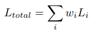
Multi-task learning concerns the problem of optimising a model with respect to multiple objectives. The naive approach to combining multi objective losses would be to simply perform a weighted linear sum of the losses for each individual task:

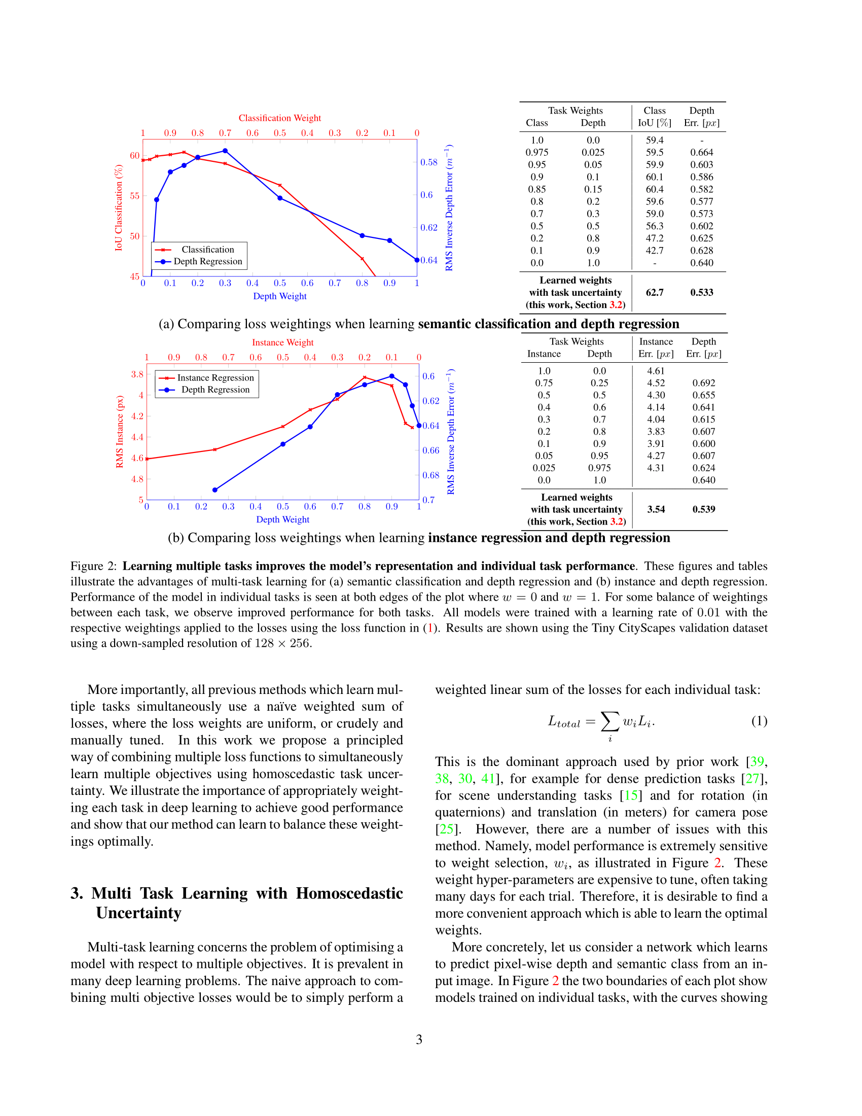
However, there are a number of issues with this method. Namely, model performance is extremely sensitive to weight selection, wi, as illustrated in Figure 2. These weight hyper-parameters are expensive to tune, often taking many days for each trial. Therefore, it is desirable to find a more convenient approach which is able to learn the optimal weights

Mathematical Formulation

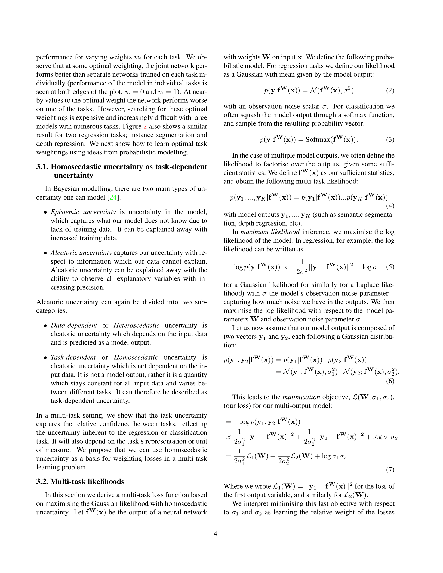
First the paper defines multi-task likelihoods:
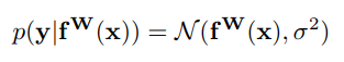
- For regression tasks, likelihood is defined as a Gaussian with mean given by the model output with an observation noise scalar σ:

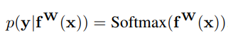
- For classification, likelihood is defined as:

where:

In maximum likelihood inference, we maximise the log likelihood of the model. In regression for example:

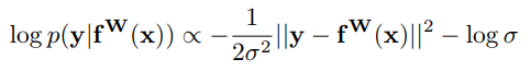
σ is the model’s observation noise parameter - capturing how much noise we have in the outputs. We then maximise the log likelihood with respect to the model parameters W and observation noise parameter σ.

Assuming two tasks that follow a Gaussian distributions:

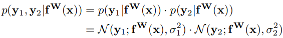
The loss will be:


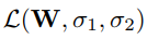
This means that W and σ are the learned parameters of the network. W are the wights of the network while σ are used to calculate the wights of each task loss and also to regularize this task loss wight.

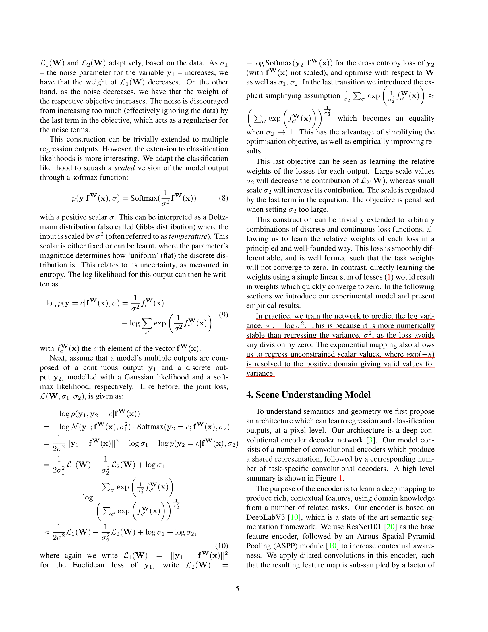
However, the extension to classification likelihoods is more interesting. We adapt the classification likelihood to squash a scaled version of the model output through a softmax function:

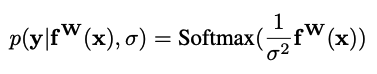
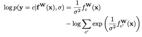
with a positive scalar σ. This can be interpreted as a Boltzmann distribution (also called Gibbs distribution) where the input is scaled by σ2 (often referred to as temperature). This scalar is either fixed or can be learnt, where the parameter’s magnitude determines how ‘uniform’ (flat) the discrete distribution is. This relates to its uncertainty, as measured in entropy. The log likelihood for this output can then be written as

assume that a model’s multiple outputs are composed of a continuous output y1 and a discrete output y2, modelled with a Gaussian likelihood and a softmax likelihood, respectively. Like before, the joint loss, L(W, σ1, σ2), is given as:

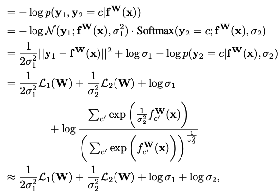
In practice, we train the network to predict the log variance, s := log σ2. This is because it is more numerically stable than regressing the variance, σ2, as the loss avoids any division by zero. The exponential mapping also allows us to regress unconstrained scalar values, where exp(−s) is resolved to the positive domain giving valid values for variance.

代码实现

def build_model(model_config):
  inputs = []
  outputs = []

  return LossesUWLModel(inputs=inputs, outputs=outputs)

class LossesUWLModel(tf.keras.Model):

    def __init__(self, *args, **kwargs):
        super().__init__(*args, **kwargs)
        self.sigma = [tf.Variable(tf.random.uniform(shape=[], minval=0.2, maxval=1, seed=10), dtype=tf.float32,
                                  trainable=True,
                                  constraint=tf.keras.constraints.NonNeg(),
                                  name=o + 'sigma') for o in self.output_names]

    def train_step(self, data):
        # Unpack the data. Its structure depends on your model and
        # on what you pass to `fit()`.
        x, y = data

        with tf.GradientTape() as tape:
            y_pred = self(x, training=True)  # Forward pass
            # Compute the loss value
            # (the loss function is configured in `compile()`)

            task_loss = []
            total_loss = 0.0
            for i in range(len(self.output_names)):
                target_name = self.output_names[i]
                loss_i = self.loss[target_name](y_true=y[target_name], y_pred=y_pred[i])
                task_loss.append(loss_i)
                total_loss = tf.add(total_loss, tf.divide(loss_i, self.sigma[i] ** 2))
                total_loss = tf.add(total_loss, tf.math.log(self.sigma[i] ** 2))

        trainable_vars = self.trainable_variables
        gradients = tape.gradient(total_loss, trainable_vars)
        # Update weights
        self.optimizer.apply_gradients(zip(gradients, trainable_vars))
        # Update metrics (includes the metric that tracks the loss)
        self.compiled_metrics.update_state(y, y_pred)

        return {m.name: m.result() for m in self.metrics}


model = build_model(FLAGS.model_config)
model.compile(
    optimizer=tf.keras.optimizers.RMSprop(FLAGS.lr),
    loss={
        "a": tf.keras.losses.BinaryCrossentropy(name='loss', label_smoothing=0.1),
        "b": tf.keras.losses.BinaryCrossentropy(name='loss'),
    },
    metrics={
        "a": [tf.keras.metrics.BinaryCrossentropy(), tf.keras.metrics.AUC(name='auc')],
        "b": [tf.keras.metrics.BinaryCrossentropy(), tf.keras.metrics.AUC(name='auc')],
    },
    # run_eagerly=True
)

论文